Visualizing Open X-Embodiment Dataset in Foxglove.

Last month, we released the Foxglove SDK, our toolkit that enables you to supercharge your integration with Foxglove, making data visualization easier than ever, regardless of your robotics software stack.
Fig. 1 Berkeley_autolab_ur5 data visualized in Foxglove.
In this tutorial, we will demonstrate how easy it is to streamline a dataset visualization using a selected Open X-Embodiment dataset.
Open X-Embodiment.
Open X-Embodiment is a dataset resulting from a collaboration among 21 institutions. The dataset demonstrates 527 skills and contains 2,419,193 episodes.
In the Open X-Embodiment Dataset Overview, you will find a list of all datasets, with a neat table showing what you can expect to see in each of them. Note that each dataset may contain different modalities that may be of interest if you would like to explore the data.
The datasets in Open X-Embodiment don’t have a fixed structure, and what you will find in the dataset depends on the Researchers who created the dataset. Because of this, you will need to approach each dataset individually, as we will in this blog post.
A good entry point to Open X-Embodiment is this jupyter notebook on colab. We will base our data fetching logic on this resource.
Tutorial.
For this tutorial, I selected the berkeley_autolab_ur5 dataset. The data contains multiple camera feeds (including a depth camera!) and plenty of robot states, making it a fun demonstrator to work with.
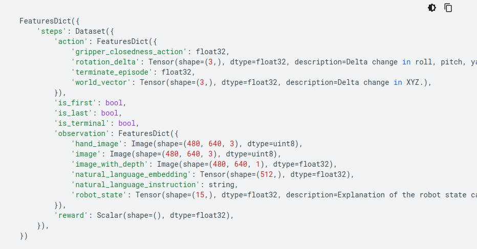
Fig.2. The feature structure that you can find on tensorflow.org is very helpful for data wrangling that we will do in this tutorial.
In this tutorial, we assume that you have Python 3.9 or later installed on your machine. You will also need to install the following Python packages:
Fetching an episode.
We will start our adventure by specifying some imports, global variables, and some code to fetch the dataset that’s based on the official colab
import tensorflow_datasets as tfds

DATASET = "berkeley_autolab_ur5"
TARGET_EPISODE = 40
CONTROL_RATE_HZ = 5  # Depends on the dataset!


def dataset2path(dataset_name):
    if dataset_name == "robo_net":
        version = "1.0.0"
    elif dataset_name == "language_table":
        version = "0.0.1"
    else:
        version = "0.1.0"
    return f"gs://gresearch/robotics/{dataset_name}/{version}"


b = tfds.builder_from_directory(builder_dir=dataset2path(DATASET))
ds = b.as_dataset(split="train[{}:{}]".format(TARGET_EPISODE, TARGET_EPISODE + 1))
episode = next(iter(ds))

print("Successfully loaded the dataset: ", DATASET)

assert "steps" in episode, "The dataset does not contain 'steps' key."
print(f"Number of steps in the episode: {len(episode['steps'])}")
In the above code, we ensure that we can fetch a dataset and that it contains an episode with some steps. When following this tutorial, you can freely select a dataset from the dataset table, but if you do, ensure that you update the CONTROL_RATE_HZ variable that we will implement in the next step.
The output we want to see when running this program is:
Successfully loaded the dataset:  berkeley_autolab_ur5
Number of steps in the episode: 114
Note that fetching the data might take some time, and you might see some warnings that you might safely ignore:
2025-06-06 11:12:09.605146: I external/local_xla/xla/tsl/cuda/cudart_stub.cc:32] Could not find cuda drivers on your machine, GPU will not be used.
2025-06-06 11:12:09.608613: I external/local_xla/xla/tsl/cuda/cudart_stub.cc:32] Could not find cuda drivers on your machine, GPU will not be used.
2025-06-06 11:12:09.618830: E external/local_xla/xla/stream_executor/cuda/cuda_fft.cc:467] Unable to register cuFFT factory: Attempting to register factory for plugin cuFFT when one has already been registered
WARNING: All log messages before absl::InitializeLog() is called are written to STDERR
E0000 00:00:1749201129.634912   33730 cuda_dnn.cc:8579] Unable to register cuDNN factory: Attempting to register factory for plugin cuDNN when one has already been registered
E0000 00:00:1749201129.640805   33730 cuda_blas.cc:1407] Unable to register cuBLAS factory: Attempting to register factory for plugin cuBLAS when one has already been registered
W0000 00:00:1749201129.657395   33730 computation_placer.cc:177] computation placer already registered. Please check linkage and avoid linking the same target more than once.
Iterating over the episode’s steps (tutorial 2).
We have our episode loaded, let’s now iterate through all the steps of the episode, and let’s make sure the data we find interesting is there. We will write a function print_step_info:
def print_step_info(step):
    print(f"Step {i}:")
    print(f"  image shape: {step['observation']['image'].shape}")
    print(f"  hand_image shape: {step['observation']['hand_image'].shape}")
    print(f"  image_with_depth shape: {step['observation']['image_with_depth'].shape}")
    print(
        f"  natural language instruction: {step['observation']['natural_language_instruction']}"
    )
    print(f"  Action rotation delta: {step['action']['rotation_delta']}")
    print(f"  Action world vector: {step['action']['world_vector']}")
    print(f"  Robot state: {step['observation']['robot_state']}")
And call it when we are iterating over the steps in our episode:
for i, step in enumerate(episode["steps"]):
    print_step_info(step)
The terminal output we should now see for each step looks like this:
Step 95:
  image shape: (480, 640, 3)
  hand_image shape: (480, 640, 3)
  image_with_depth shape: (480, 640, 1)
  natural language instruction: b'pick up the blue cup and put it into the brown cup. '
  Action rotation delta: [0. 0. 0.]
  Action world vector: [0. 0. 0.]
  Robot state: [-2.975159   -1.2078403   1.7616024  -2.044398   -1.7078537   3.1259193
  0.53834754  0.16683726  0.02349306  0.6345158   0.76873034 -0.07564076
  0.02686722  1.
If you’ve made it this far, great! We are now sure we can access our episode data and start streaming it!
Hello Foxglove.
We are now ready to start streaming our data to Foxglove in real time. To begin, we will ensure that the robot in our dataset actually performs the assigned tasks.
Let’s start by adding some imports that we will utilize in this section
import tensorflow_datasets as tfds
import foxglove
from foxglove import Channel
from foxglove.schemas import (
	RawImage,
)
from foxglove.channels import RawImageChannel
import time
Let’s start the Foxglove server using our SDK:
server = foxglove.start_server() # We can start it before fetching tfds datasetNow, let’s define the schema for a language instruction and a corresponding channel:
language_instruction_schema = {
    "type": "object",
    "properties": {
        "text": {
            "type": "string",
        },
    },
}
language_instruction_chan = Channel(
    topic="/natural_language_instruction", schema=(language_instruction_schema)
)
Before we proceed, let’s discuss some terminology:
- A schema describes the structure of a message’s contents. Foxglove defines several schemas with visualization support, and users can define custom schemas using supported encodings.
- A channel provides a way to log related messages sharing the same schema. Each channel is identified by a unique topic name. For Foxglove schemas, the SDK offers type-safe channels for logging messages with a known, matching schema
In short, we have created a schema for language instruction that includes a text entry, and we will publish it on the /natural_language_instruction topic.
Now, let’s modify our initial iteration through the episode steps in the following way:
- We will nest it in a while loop, to keep replaying the episode over and over
- The while loop will be nested in a try-except block to capture a keyboard interrupt
- At the end of our for loop, we will add a sleep instruction to match our control rate so that the episode is replayed at the same frequency as it was captured
- We will create the language instruction message and log it on our channel
try:
    while True:
        for i, step in enumerate(episode["steps"]):
            print_step_info(step)

            # Publish the natural language instruction
            instruction_str = (
                step["observation"]["natural_language_instruction"]
                .numpy()
                .decode("utf-8")
            )
            instruction_msg = {"text": instruction_str}
            language_instruction_chan.log(instruction_msg)

            # Publish the image
            image_msg = RawImage(
                data=step["observation"]["image"].numpy().tobytes(),
                width=step["observation"]["image"].shape[1],
                height=step["observation"]["image"].shape[0],
                step=step["observation"]["image"].shape[1] * 3,  # Assuming RGB image
                encoding="rgb8",
            )
            image_chan.log(image_msg)

            time.sleep(1 / CONTROL_RATE_HZ)

except KeyboardInterrupt:
    print("Keyboard interrupt received. Will stop the server.")
finally:
    server.stop()
    print("Server stopped.")
You can run the code now, and assuming the loop is constantly running, we will open Foxglove and connect to our server by selecting the “Open connection” button in the dashboard
Fig. 3 Connecting Foxglove to our server.
If everything went well, you will see at the top bar that Foxglove connected to the local server at ws://localhost:8765 and the current time is displayed. With Foxglove connected, we can now add a display for our natural language instruction, which will be shown in a Raw Messages panel.
Fig. 4 Adding a RawMessage and displaying our instruction in it.
Great, now we can display our instruction inside a Raw Messages panel, but the text being static throughout the episode duration hardly makes for an exciting demo. Let’s view some camera feeds.
We will start by creating a RawImageChannel for the topic /image outside our loops:
image_chan = RawImageChannel(topic="/image")Inside our iteration through the episode steps, we will now create a RawImage object and publish it on the channel we made in the previous code snippet:
# Publish the image
image_msg = RawImage(
    data=step["observation"]["image"].numpy().tobytes(),
    width=step["observation"]["image"].shape[1],
    height=step["observation"]["image"].shape[0],
    step=step["observation"]["image"].shape[1] * 3,  # Assuming RGB image
    encoding="rgb8",
)
image_chan.log(image_msg)

time.sleep(1 / CONTROL_RATE_HZ)
In this snippet, it’s crucial that we correctly assign the step value of the RawImage that calculates the row stride sizes. For an RGB8 image, this means we multiply the width by 3 channels. If we were dealing with a depth image with float32 values with 32FC1 encoding, we would multiply the width by 4 bytes.
Since our image is now being published, let’s add it to our visualization:
Fig. 5 Adding an Image panel.
Now, that’s far more exciting! Remember that the dataset we selected also has the following image feeds:
- steps/observation/hand_image (RGB8)
- steps/observation/image_with_depth (32FC1)
So you have even more room to make things dynamic in your panels
Add more visualizations (tutorial_04).
Let’s make our visualization even more exciting by adding two more elements:
- A 3D panel that will show a transform between the base of the robot and the end-effector
- A value that we can plot
Reading the dataset website, we can learn that the step/observation/robot_state contains the following information:
robot_state: np.ndarray((L, 15))
- This stores the robot’s state at each timestep.
- [joint0, joint1, joint2, joint3, joint4, joint5, x,y,z, qx,qy,qz,qw, gripper_is_closed, action_blocked]
- x,y,z, qx,qy,qz,qw is the end-effector pose expressed in the robot base frame
- gripper_is_closed is binary: 0 = fully open; 1 = fully closed
- action_blocked is binary: 1 if the gripper opening/closing action is being executed and no other actions can be performed; 0 otherwise.
Having values of x, y, z, qx, qy, qz, and qw makes it trivial for us to create a transform. We will start by updating the imports:
import tensorflow_datasets as tfds
import foxglove
from foxglove import Channel
from foxglove.schemas import (
    RawImage,
    FrameTransform,
    Vector3,
    Quaternion,
)
from foxglove.channels import (
    RawImageChannel,
    FrameTransformChannel,
)
import time
Then, we can create the FrameTransformChannel:
transform_chan = FrameTransformChannel(topic="/tf")Afterwards, we can craft a FrameTransform message and log it:
# Publish the end-effector transform
robot_state = step["observation"]["robot_state"].numpy()
transform_msg = FrameTransform(
    parent_frame_id="robot_base",
    child_frame_id="end_effector",
    translation=Vector3(
        x=float(robot_state[6]),
        y=float(robot_state[7]),
        z=float(robot_state[8]),
    ),
    rotation=Quaternion(
        x=float(robot_state[9]),
        y=float(robot_state[10]),
        z=float(robot_state[11]),
        w=float(robot_state[12]),
    )
)
transform_chan.log(transform_msg)
The FrameTransform message is simple; we specify two frames and provide translation and rotation from the parent frame to the child frame. Since the measurement units in the dataset are in the metric system and rotations are represented as quaternions, we don’t need to modify the data in any way to make it usable.
With the above change, we can add a 3D panel to our scene and visualize the transform:
Fig. 6 Frame Transforms in 3D panel.
Now, for the plotting of float value, we will create a custom schema:
float_schema = {
    "type": "object",
    "properties": {
        "value": {
            "type": "number",
            "format": "float",
        },
    },
}
And we will create a Channel object using this schema, just like we did for the natural language instruction at the beginning of this tutorial:
gripper_chan = Channel(
    topic="/gripper_state",
    schema=(float_schema)
)
To log the gripper status, we can now do the following:
# Publish the gripper state
gripper_msg = {"value": float(robot_state[13])}
gripper_chan.log(gripper_msg)
Adding a plot panel to Foxglove, we can now drag and drop the gripper_state value from the Topics tab to the plot panel, and we will be able to display the state as follows:
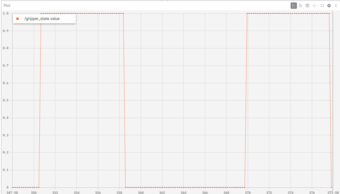
Fig. 7. A plot panel showing the gripper_status value.
Recording data as MCAP.
We are now approaching my favorite part of the SDK implementation, recording data for future replay. It could not be any simpler:
filename = f"{DATASET}_episode_{TARGET_EPISODE}.mcap"
writer = foxglove.open_mcap(filename)
server = foxglove.start_server()
We construct a filename that will hold a meaningful name for us, and create a writer object. That’s it. Now, all the data we log will also be saved to the MCAP file.
Before we run this code, we should comment out our while loop; after all, we want our MCAP to contain a single episode.
We now invite you to experiment with the datasets, log even more data, and create your own layout.
As for me, here is my current setup for this dataset:
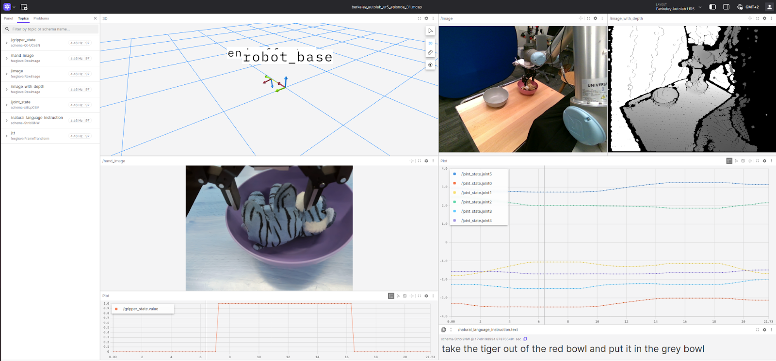
Fig. 8 Mat’s layout for the Berkeley Autolab UR5 dataset.
If you’d like to reuse my layout, or view the source code, please check out our tutorials repository.
Want to take it further?
In this tutorial, we discussed the basics of Foxglove SDK in Python. The code we’ve built is a great starting point for you to explore Open X-Embodiment and other datasets. Here are some ideas on what you can do next (consider this homework):
- Write code to log other images present in the dataset, including the depth image
- Load another dataset and repeat the steps we performed on it (you will notice that the structure differs between datasets, so you will need to make some adjustments)
- Load the UR5 model and use the joint angles to represent the robot state
- Modify the code to load more episodes and log them to a single MCAP file
- When logging to MCAP, remove the call to sleep, and instead manually provide the timing information to convert to MCAP without needing to wait for each episode to play out