Announcing: “custom timestamp field” in the Plot and State Transitions panels.
Plotting temporal data in Foxglove with flexibility.


Foxglove now lets you choose an arbitrary timestamp field from your messages when plotting data, giving you more control over how time-based data is visualized. While standard log time is still required for indexing and playback—such as receive time in ROS or timestamp in ULog—the Plot and State Transitions panels support MCAP publish time, ROS header stamps, and custom fields from any part of a message. This flexibility helps eliminate time skew, improves clarity, and allows you to visualize data in a way that best reflects the real-world events your robots experienced.
When and why to use custom time.
Robotics systems often deal with multiple timestamps, for example:
- Log time: The time a central logger records the message. This is often close to wall-clock time but can be skewed by network latency or buffering.
- Publish time: The time a message was created, usually closer to the actual event.
- ‘Other’ time: A timestamp pulled from an arbitrary part of the message, often designed to reflect domain-specific timing details.
Foxglove’s custom timestamp capability allows you to extract timestamps from deep within the message data. These timestamps can represent highly specific events, such as:
- The time a sensor captured an image or scan.
- The exact moment an actuator began moving.
- A timestamp synchronized with external systems, such as GPS or motion capture.
By using custom time, you’re no longer constrained by the limitations of log time or publish time. Instead, you can align your data in the Plot and State Transitions panels to the time axis that matters most for your application.
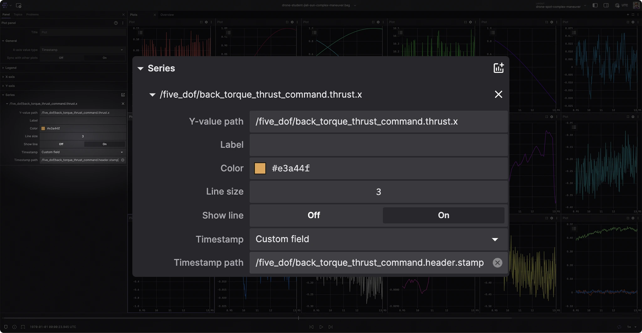
The Foxglove UI showing the new Custom field for Timestamp and Timestamp path.
Note: an important caveat to keep in mind when using custom timestamps or alternative time sources in Foxglove’s Plot and State Transitions panels is that the “current playback time” shown in the playback bar—and across all other panels—is based on log time. For example, if you scrub to a specific point in time and compare a value in a plot using a custom timestamp with the same value in the Raw Messages panel, the two may not align.
Making sense of time.
Time in robotics is rarely straightforward. A single system might juggle an operating system clock, a high-resolution hardware timer, and a GPS clock, each with its quirks. Add to that the fact that different parts of your system might interpret “now” differently—did “now” happen when the photon hit the camera sensor? When the image was written to disk? Or when it was processed downstream? Monotonic or wall time? And with what epoch definition?
Protocols and recording formats like MCAP, ROS bags, and ULog offer various built-in and user-defined methods for storing timestamps, but they differ widely in how clearly they define the interpretation of those timestamps. This lack of consistency can create real challenges when analyzing or synchronizing data across different sources, especially in robotics systems that depend on precise timing. These issues aren’t just theoretical—they directly impact tasks like debugging sensor fusion algorithms or replaying logs for simulation, where even slight timestamp mismatches can lead to confusing, misaligned plots and misleading conclusions.
MCAP, for example, defines two key timestamps: ‘log time’, which marks when a central logger received the message, and ‘publish time’, when the message was originally created by a node. Although publish time is usually closer to the real-world event, MCAP indexes data using log time, often leading to playback artifacts that distort the time-series view. Similar issues arise in ROS, where developers contend with receipt time and header stamps. In fast-moving or multi-sensor systems, choosing the wrong timestamp can obscure cause-and-effect relationships and make debugging unnecessarily difficult.
Harnessing time for better insights.
Working with temporal data in robotics isn’t just about collecting timestamps or aligning plots—it’s about choosing the right timestamp for the job to ensure accurate analysis, faster debugging, and a deeper understanding of your system. The timestamp you use should ideally approximate a universal “wall time” to minimize discrepancies caused by network latency, batching, or buffering.
Foxglove gives you the flexibility to select the most meaningful time reference for your data—whether that’s log time, publish time, or a custom timestamp field—so you can visualize and interpret events as they truly happened. Note: for greater consistency across your datasets, it may be worth pre-processing and normalizing your message log times before uploading to Foxglove, ensuring coherent playback and more reliable insights.
So, the next time you’re staring at a misaligned plot, remember: time is on your side—you just need to know how to use it and have the flexibility to do so.