Grids and Voxels: adding the 3rd dimension.


Foxglove now supports full 3D visualization of grid_map_msgs/GridMap and costmap_2d/VoxelGrid messages. Until now, grids in Foxglove were limited to flat textured planes using Occupancy Grids or our own Grid format. But grid maps are a cornerstone of modern robotic perception, enabling you to encode and reason about complex surfaces—from terrain elevation and surface normals to friction coefficients and foothold quality. With these updates, Foxglove can natively render richer maps, so you can explore elevation data, voxel-based costmaps, and multi-layered surface information directly in the 3D panel.
Whether you’re building autonomous navigation for rough terrain or debugging your perception stack, you’ll gain deeper spatial insight with minimal setup.
Elevation.
When we sample colors from a grid message’s fields or layers, depending on the message schema, the most straightforward way to add a third dimension is to displace the grid perpendicular to its surface using values from another field or layer. There are several ways to interpret that displacement and interpolate between data points. In Foxglove, we’ve chosen to support the following methods, shown here using an example grid.
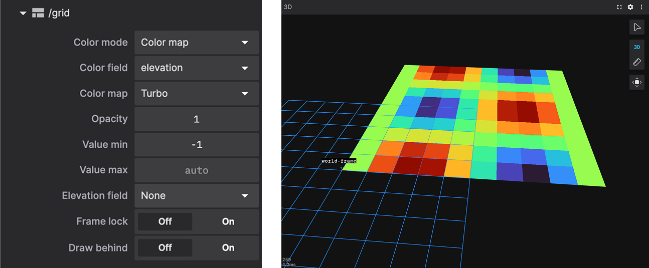
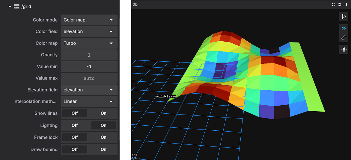
Linear.
The simplest approach is linear interpolation between elevation values. In this method, you subdivide the plane into an N×M grid that matches the resolution of your elevation data, then use a vertex shader to displace each vertex accordingly.
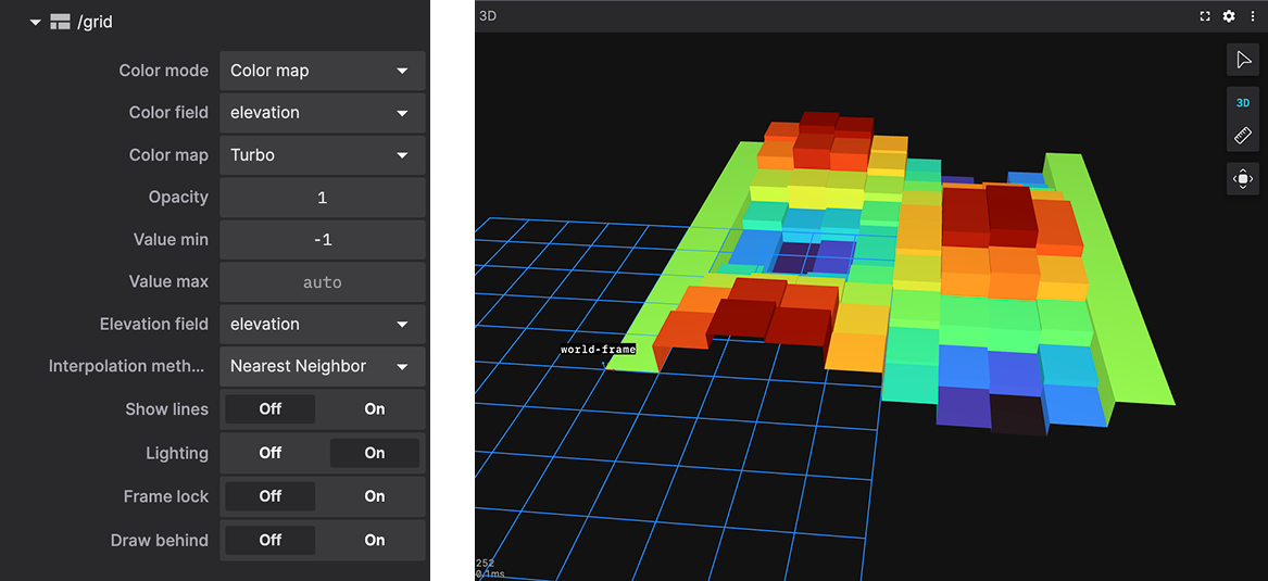
Nearest neighbor.
A more complex interpolation method is nearest neighbor. This approach represents each elevation data point as an adjacent cuboid, with the undersides left unrendered. Because each data point now consists of multiple vertices, you need to consider how to render them on the GPU while minimizing mesh updates on the CPU for each new message received on a topic.
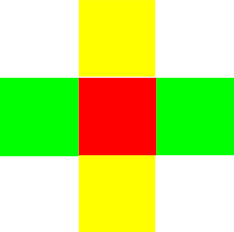
If you break down a single data point and its box-like shape, you can unwrap it into the following layout: red represents the data point itself, green shows the cuboid’s sides along the X axis, yellow shows the sides along the Y axis, and white indicates unused space.
Since we’re only displaying the elevation differences between data points, we can share sides between adjacent points to avoid rendering duplicate geometry.
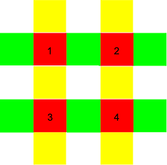
By discarding sides we don’t need, such as the outer edges, we can create a uniform tiling pattern that resembles a grid twice the size of the original elevation data. In practice, the bottom row and right column would also be removed as outer edges, but this example simply illustrates the tiling pattern you’d see.
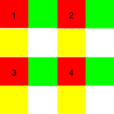
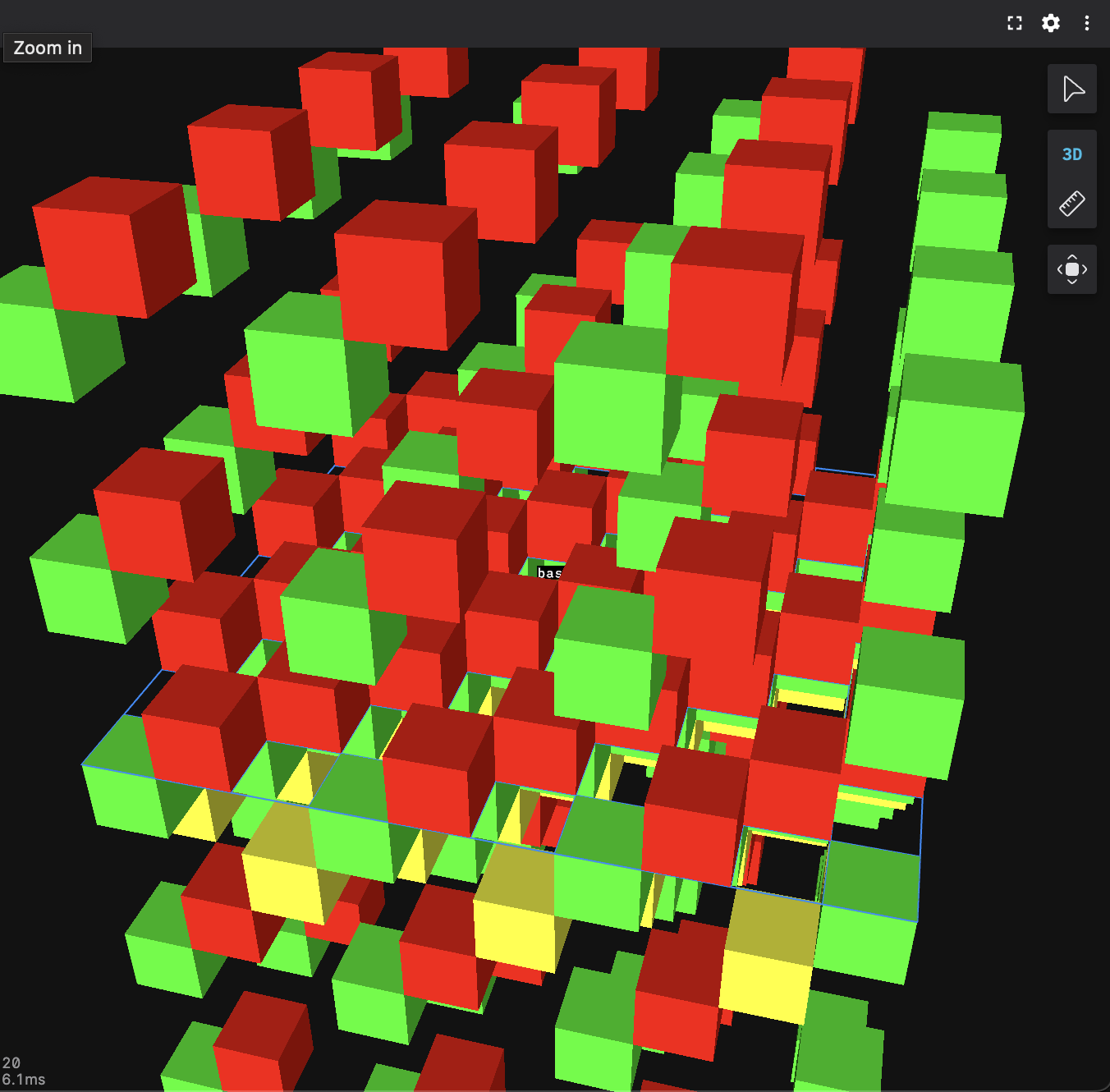
With this approach, you can use a vertex shader to fold the red squares so they sit adjacent along the X and Y axes, then displace them along the Z axis based on their elevation. The final result looks something like this.
Voxels.
If the 3D data you need to represent is sparse or non-adjacent, the new voxel visualization options may be a better fit than grid-based elevations.
Grid.
Voxel grids extend the concept of 2D grids by adding a third dimension, creating a volume of size N×M×K. The ROS VoxelGrid format is an exception, it uses a single uint32 to encode voxel states, with the top and bottom 16 bits indicating whether a cell is marked or present. This limits the grid to a maximum size of NxMx16.
Given that the data of a voxel grid between messages can entirely change, generating all the geometry on the CPU or running change detection every frame would be too resource-intensive. Instead, we use shaders that implement a variation of the digital differential algorithm (DDA). This approach lets the shader work directly with the raw 3D data, ray marching through the voxel volume on a per-pixel basis until it hits a populated cell to draw. If the cell is transparent, the shader keeps marching but blends colors as it goes.
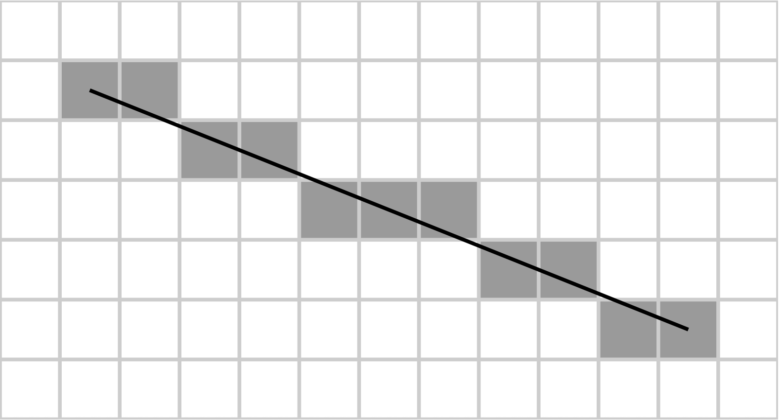
2D example of a ray stepping through the voxel volume.
Point cloud.
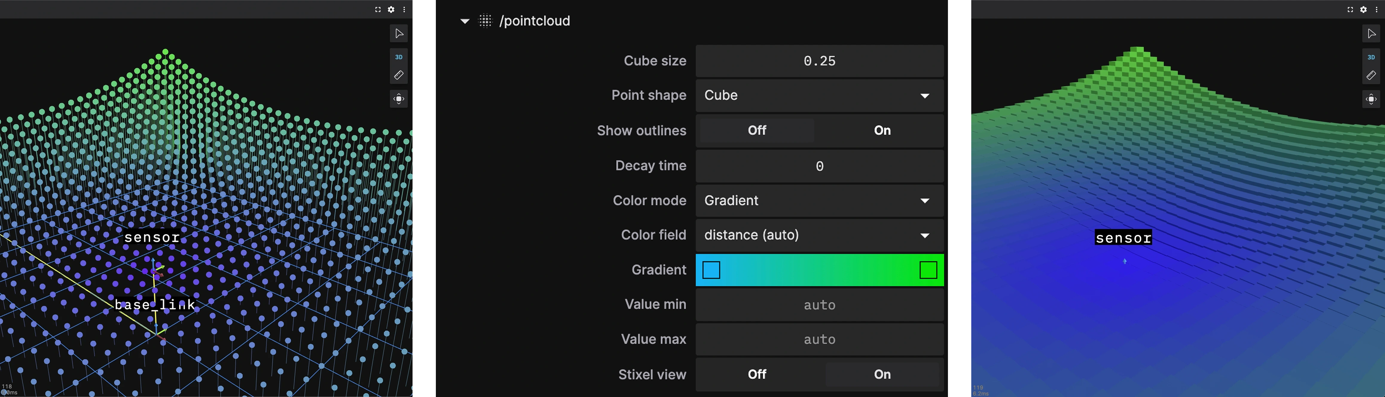
We’ve also added a new setting to render points as cubes in point clouds, giving the data a volumetric appearance. Since point distribution isn’t guaranteed to follow a uniform grid, all cubes are rendered as instances of a single cube mesh. If the points do happen to align uniformly in 3D space, the result will look similar to a voxel grid.
Wrapping up.
With these changes, visualizing three dimensional data is now possible. Check out the following documentation for the specifics:
The 3D panel is designed to visualize all your data types without blind spots, reflecting Foxglove’s broader mission to deliver the most performant and comprehensive platform for developing Physical AI. Whether you’re focused on perception, control, simulation, or full-system integration, Foxglove helps you understand your robots more deeply, debug faster, and build reliable autonomy with confidence.
Sign up here to get started for free today.