Comparing ML training using the Foxglove SDK.


In this tutorial we are going to use Foxglove SDK to load a dataset of autonomous navigation driving to compare different runs of the unmanned robot.
The dataset contains information such as run_id, timestamp, min and max detection of the lidar, position and time taken. In addition to this data, we will infer some additional values such as speed: traveled distance divided by time taken.
Let’s take a look at a row from the dataset:
The run_id column contains the ID of the run. The timestamp is the instant of time of the row. lidar_min and lidar_max are the min and max values of the lidar read at that moment, the same with ultrasonic_left and ultrasonic_right are the read values of the ultrasonic sensor.
The x and y value are the position in that moment, the same with orientation in degrees. Additional information in the row is the battery_level in percentage, the collision_flag which represents if there is a collision.
The path_smoothness is a value in the range 0 to 1 which represents how smooth the path is, being 1 the most smooth. Finally, time_taken are the seconds to reach the target, which is also a column that contains the result of the run: success, collision, partial, and timeout.
run_id
timestamp
lidar_min
lidar_max
ultrasonic_left
ultrasonic_right
x
y
orientation
1
0
0.76
3.04
0.97
1.63
0.13
0.1
316.54
battery_level
collision_flag
path_smoothness
time_taken
target
98.9
0
0.83
34
timeout
A quick glance at the dataset reveals many rows, with many rows and timestamps for each data read. Using the foxglove_sdk we will generate a MCAP file to visually compare the runs.
Previous steps.
The dataset is provided in the following link. Download the CSV file and save it in a folder with the following structure:
- autonomous_indoor
- code
- data
- autonomous_navigation_dataset.csv
The code.
Start by creating a new Python file named generate_mcap.py in the code folder. Import the necessary modules that will be used. Define variables for the folders.
import os
import csv
import math

import foxglove
from foxglove import Channel
from foxglove.schemas import (
    Pose,
    PoseInFrame,
    Vector3,
    Quaternion,
    Timestamp,
    PosesInFrame,
    KeyValuePair,
    LaserScan,
    FrameTransform,
    LinePrimitive,
    SceneEntity,
    SceneUpdate,
    Color,
    Point3
)
from foxglove.channels import (
    PoseInFrameChannel,
    PosesInFrameChannel,
    KeyValuePairChannel,
    LaserScanChannel,
    FrameTransformChannel,
    SceneUpdateChannel
)

ROOT_DIR = os.path.abspath(os.path.join(os.path.dirname(__file__), ".."))
CSV_FILE = os.path.join(ROOT_DIR, "data", "autonomous_navigation_dataset.csv")
OUTPUT_FOLDER = os.path.join(ROOT_DIR, "output")
os.makedirs(OUTPUT_FOLDER, exist_ok=True)
OUTPUT_FILE = os.path.join(OUTPUT_FOLDER, "autonomous_navigation_dataset.mcap")
Create a variable for assign colors depending on the result of the run. There are 4 possible results: “collision”, “success”, “partial” and “timeout”. Define 4 RGB colors in float format.
COLOR_BY_RESULT = {
    "collision": (1.0, 0, 0),  # Red
    "success": (0, 1.0, 0),  # Green
    "partial": (0, 0, 1.0),  # Blue
    "timeout": (1.0, 1.0, 0),  # Yellow
}
Auxiliary functions.
Clean code programming include structuring the program into simple functions that make the code readable, unit-testable and easier to maintain.
The first function to define is used to convert from Roll, Pitch and Yaw (RPY) angles to a Quaternion. The RPY angles are easier for a human to understand, whereas the quaternion is more efficient for mathematical operations.
def rpy_to_quaternion(roll: float, pitch: float, yaw: float) -> tuple[float, float, float, float]:
    """Convert roll, pitch, yaw angles to quaternion."""

    cy = math.cos(yaw * 0.5)
    sy = math.sin(yaw * 0.5)
    cr = math.cos(roll * 0.5)
    sr = math.sin(roll * 0.5)
    cp = math.cos(pitch * 0.5)
    sp = math.sin(pitch * 0.5)

    w = cy * cr * cp + sy * sr * sp
    x = cy * sr * cp - sy * cr * sp
    y = cy * cr * sp + sy * sr * cp
    z = sy * cr * cp - cy * sr * sp

    return (x, y, z, w)
The next function is a simple method to open a CSV file and return the contents as a list of rows. Each column can be accessed like a Python dictionary.
def open_csv(file_path: str) -> list[dict]:
    """
        Open a CSV file and return its contents as a list of dictionaries
        Input:
            file_path (str): Path to the CSV file
        Output:
            list[dict]: List of dictionaries representing the CSV rows

    """
    with open(file_path, "r", encoding="utf-8") as file:
        csv_reader = csv.DictReader(file)
        fields = csv_reader.fieldnames
        data = list(csv_reader)
    print(f"Available data fields: {fields}")
    return data
As explained before, each row contains information about the robots position for each run. The next function will use this information to generate messages information, using the data from columns x and y. Additional data is created, such as the orientation between positions and the speed. The output of this function is the pose in Pose message, the Frame message and finally, the speed data in float.
def get_pose_and_speed(timestamp, row, prev_ts, prev_position) -> None:
    ts = timestamp.sec
    # Create the messages starting from the basic ones
    position = Vector3(
        x=float(row["x"]),
        y=float(row["y"]))
    # Calculate orientation based on previous position
    yaw = math.atan2(
        float(row["y"]) - prev_position[1],
        float(row["x"]) - prev_position[0])
    quat = rpy_to_quaternion(
        roll=0,
        pitch=0,
        yaw=yaw)
    orientation = Quaternion(x=quat[0], y=quat[1], z=quat[2], w=quat[3])
    # Calculate speed based on traveled distance divided by time taken
    if ts > 0:
        speed = math.sqrt(
            (float(row["x"]) - prev_position[0]) ** 2 +
            (float(row["y"]) - prev_position[1]) ** 2) / (ts-prev_ts)
    # First instance or if ts is 0, set speed to 0
    else:
        speed = 0.0

    pose = Pose(
        position=position,
        orientation=orientation
    )

    frame = FrameTransform(
        timestamp=timestamp,
        parent_frame_id="odom",
        child_frame_id=f"id_{row['run_id']}",
        translation=position,
        rotation=orientation
    )

    return pose, speed, frame
The next function will also use the x and y data from the row, but the message created will be displayed a SceneEntity in Foxglove’s 3D panel. Leveraging all the types of SceneEntity increases the methods of representing data and therefore, understanding the robot’s behavior. In this case, the LinePrimitive is used to display the robot’s path at each moment.
def get_line_scene(row, pts: list) -> tuple[SceneEntity, list]:
    pt = Point3(
        x=float(row["x"]),
        y=float(row["y"]),
        z=0
    )

    if row["timestamp"] == '0':
        pts[row['run_id']].clear()
    pts[row['run_id']].append(pt)

    color = COLOR_BY_RESULT[row["target"]]
    line = LinePrimitive(
        points=pts[row['run_id']],
        color=Color(r=color[0], g=color[1], b=color[2], a=1.0),
        thickness=0.05
    )

    line_entitity = SceneEntity(lines=[line],
                                id=f"id_{row['run_id']}",
                                frame_id="odom",
                                metadata=[KeyValuePair(
                                    key="target",
                                    value=row["target"]),
                                    KeyValuePair(
                                    key="time_taken",
                                    value=row["time_taken"])])

    return line_entitity, pts
The main function.
The final function to create is the generate_mcap. This function will act as the main function in our code. The first thing is to create the MCAP writer using foxglove_sdk module. Then, read the CSV data using the function previously defined.
def generate_mcap() -> None:
    writer = foxglove.open_mcap(
        OUTPUT_FILE, allow_overwrite=True)

    data = open_csv(CSV_FILE)
The next step is to define all the channels used to publish messages. For each message, we will use a dictionary to store the message for the run_id. Each channel is then created associated to the key run_id and we will be able to select each topic using this information. Additionally, some channels are not dependent on the run_id , so no dictionary is needed. Other channels are defined using the possible results of the run.
    # A channel will be created for each run_id
    pose_channels = {}
    poses = {}
    poses_channels = {}
    battery_channels = {}
    path_smoothness_channels = {}
    laser_channels = {}
    ultrasound_channels = {}
    frames_channels = {}
    pts = {}
    speed_channel = {}

    # Initialize channels for each run_id
    for row in data:
        pose_channels[row['run_id']] = PoseInFrameChannel(
            f"{row['run_id']}/pose")
        poses_channels[row['run_id']] = PosesInFrameChannel(
            f"{row['run_id']}/path")
        poses[row['run_id']] = []
        battery_channels[row['run_id']] = Channel(
            f"{row['run_id']}/battery")
        path_smoothness_channels[row['run_id']] = KeyValuePairChannel(
            f"{row['run_id']}/path_smoothness")
        laser_channels[row['run_id']] = LaserScanChannel(
            f"{row['run_id']}/laser")
        ultrasound_channels[row['run_id']] = LaserScanChannel(
            f"{row['run_id']}/ultrasound")
        frames_channels[row['run_id']] = FrameTransformChannel(
            f"{row['run_id']}/tf")
        speed_channel[row['run_id']] = Channel(
            f"{row['run_id']}/speed")

        pts[row['run_id']] = []

    target_result_channels = Channel("/target_result")
    time_taken_channel = Channel("/time_taken")

    scene_channels = {}
    scene_entities = {}
    results_count = {}
    results_channel = Channel("/results")
    possible_results = set(row['target'] for row in data)

    for result in possible_results:
        scene_entities[result] = []
        scene_channels[result] = SceneUpdateChannel(f"{result}/scene")
        results_count[result] = 0
Once all the channels have been defined, initialize variables before iterating over the rows. The target_results list will contain the results for each run, and will be published later. The prev_ variables store the previous value of run_id , position and timestamp ts.
In the iteration process, get the values from the rows using the key elements of the columns. Using the defined functions helps understand the code better. For each row, the pose , speed and frame are stored then published. The same with the lines that will be displayed in the 3D panel. Additional data is published in diverse methods. For example, the speed is published using the JSONSchema directly, which is like a Python dictionary. However, path_smoothness value is published as a KeyValue element. Both methods are correct and will be properly displayed in Foxglove. This tutorial shows both to understand how each of them is used.
    target_results = []
    prev_id = '0'
    prev_position = (0, 0)
    prev_ts = 0

    # Iterate through the data and create the necessary messages
    for row in data:
        # Get timestamp as float and convert to Timestamp
        ts = float(row["timestamp"])
        timestamp = Timestamp(sec=0, nsec=0).from_epoch_secs(ts)

        # Clear previous data if 'run_id' has changed
        if prev_id != row['run_id']:
            scene_entities[row["target"]].clear()
            prev_position = (0, 0)

        # Get the pose, speed and frame for the current row
        pose, speed, frame = get_pose_and_speed(
            timestamp, row, prev_ts, prev_position)

        # Log the pose, poses (path), frame and speed
        pose_stamped = PoseInFrame(
            pose=pose, frame_id="odom", timestamp=timestamp)
        pose_channels[row['run_id']].log(pose_stamped, log_time=int(ts*1e9))

        poses[row['run_id']].append(pose)
        poses_frame = PosesInFrame(
            timestamp=timestamp, frame_id="odom", poses=poses[row['run_id']])
        poses_channels[row['run_id']].log(poses_frame, log_time=int(ts*1e9))

        speed_channel[row['run_id']].log(
            {"speed": speed}, log_time=int(ts*1e9))

        frames_channels[row['run_id']].log(frame, log_time=int(ts*1e9))

        # Create the scene entity for the current row
        scene_entity, pts = get_line_scene(row, pts)

        # Append, log the scene entity and update the scene
        scene_entities[row["target"]].append(scene_entity)
        scene_channels[row["target"]].log(SceneUpdate(entities=scene_entities[row["target"]]),
                                          log_time=int(ts*1e9))

        # Log other data

        # Battery as JSONSchema directly
        battery = {"battery": row["battery_level"]}
        battery_channels[row["run_id"]].log(battery, log_time=int(ts*1e9))

        # Time taken as JSONSchema with X value 'run_id' and Y value 'time_taken'
        time_taken_channel.log(
            {"run_id": int(row["run_id"]),
             "time_taken": int(row["time_taken"])}, log_time=int(ts*1e9))

        # Path smoothness as KeyValuePair
        path_smoothness = KeyValuePair(
            key="path_smoothness", value=row["path_smoothness"])
        path_smoothness_channels[row["run_id"]].log(
            path_smoothness, log_time=int(ts*1e9))

        # Ultrasound scan as LaserScan in angles -90 and 90 degrees
        ultrasound_scan = LaserScan(
            timestamp=timestamp,
            frame_id=f"id_{row['run_id']}",
            start_angle=-3.141592/2,
            end_angle=+3.141592/2,
            ranges=[float(row["ultrasonic_right"]),
                    float(row["ultrasonic_left"])],
            intensities=[0, 100],
        )
        ultrasound_channels[row["run_id"]].log(
            ultrasound_scan, log_time=int(ts*1e9))

        # Register the results and count each result
        target_results.append(row["target"])
        results_count[row["target"]] += 1

        # Store the previous id, timestamp and position
        prev_id = row['run_id']
        prev_ts = ts
        prev_position = (float(row["x"]), float(row["y"]))

    target_result_channels.log(
        {"results": target_results}, log_time=int(0*1e9))
    results_channel.log(
        results_count, log_time=int(0*1e9))


if __name__ == "__main__":
    generate_mcap()
Now the code is ready to be executed. Run the code with Python and a new folder called output will appear with the .mcap file inside.
Building the layout.
Open the .mcap file with Foxglove and start a new layout. Add a 3D panel and hide all transformations, as there are too many to see clearly. Select the odom frame and one of your choosing, for example, id_1. Visualize the path of the same id searching for the topic 1/path .
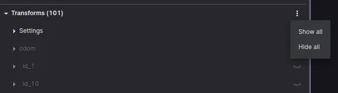
Hide all transforms.
Hide all transforms.
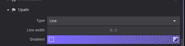
Visualize the path.
Visualize the path.
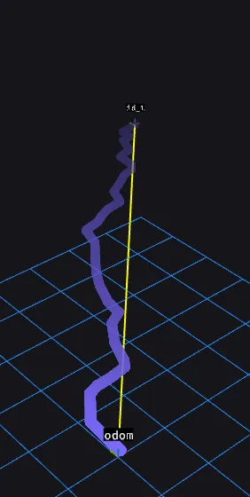
The path visualized.
The path visualized.
Open a new 3D panel to visualize all the paths at the same time using the Lines as SceneEntities. Search in the panel configuration the word scene to see all topics with the SceneEntities. Select the success/scene to see all runs that succeeded. Open as much 3D panels as you like to visualize paths and lines.
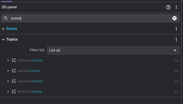
Searching for scene topics.
Searching for scene topics.
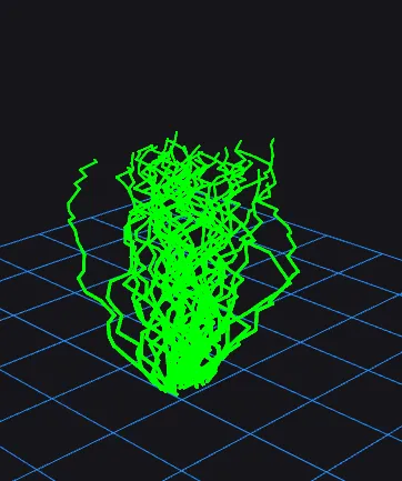
Success lines.
Success lines.
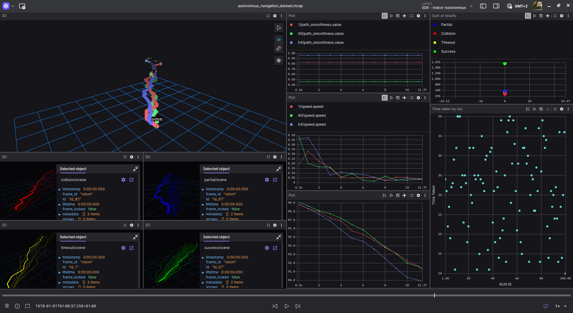
The next message to visualize is the time_taken by run_id. Keep in mind this plot is not time-related, but a XY plot. Configure the X-axis value type as Message path. Then select to plot the topic and select the X-value path as /time_taken.run_id and the Y-value as /time_taken.time_taken.
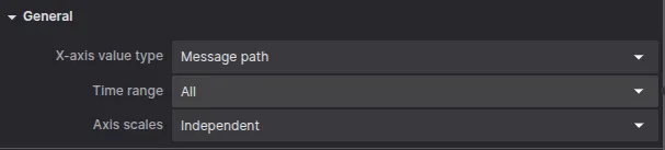
Select X-axis value type.
Select X-axis value type.
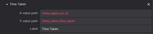
Select time_taken topic elements.
Select time_taken topic elements.
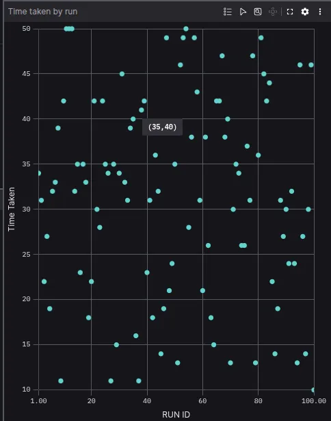
The resulting plot will represent the time taken by each run id. In the following image, the run id 35 took 40 seconds. In this case, there appears to be no relation between the run_id and the time taken.
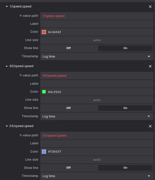
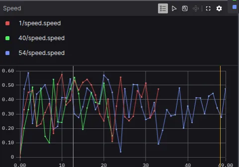
An additional plot to represent is the speed of each run. Open a new plot and select the topic n/speed , where n represent whichever run_id. For example, plot speeds for run_ids 1, 40 and 54.
Play around the different panels to understand new methods of visualizing data that can reduce your debugging time and accelerate your robotics development.
Reference layout.
The layout used in the front image of the post can be used as a reference.
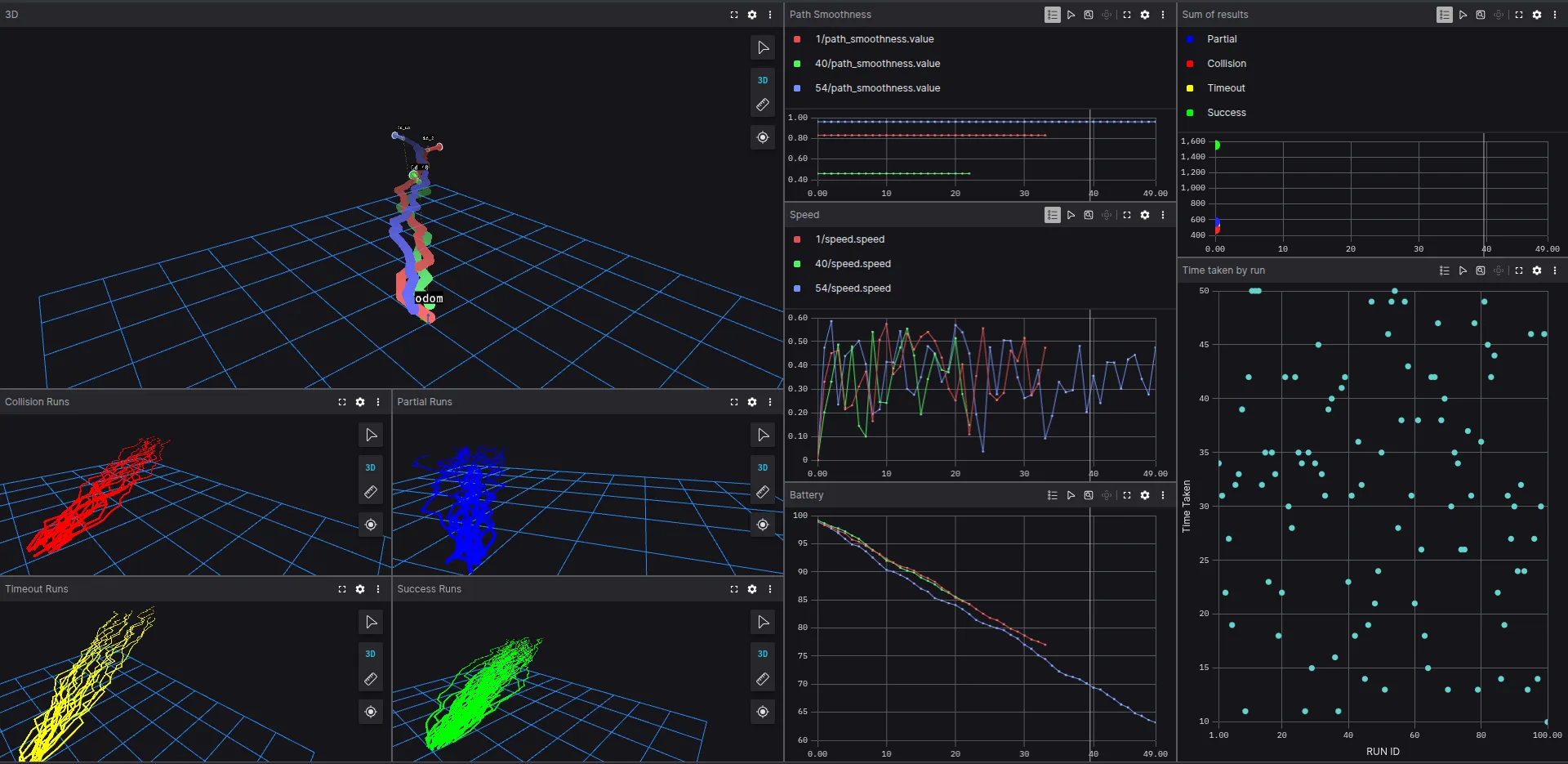
The ML training visualized using Foxglove.
The ML training visualized using Foxglove.
Keep on learning.
In this tutorial we have used a simple CSV file, which could be produced by a budget-friendly robot, and visualized the data in Foxglove. The dataset contains several runs with different results.
Foxglove can be used to compare multiple training sessions and results of a machine learning algorithm related to unmanned ground vehicles, aerial robots or humanoid learning to walk.
Join our community and keep in touch to learn more about this new tool that will help you log better data from your robots, learning about their behavior both in real time and after.