Converting the LAFAN1 Retargeting dataset to MCAP.


This tutorial shows how to convert the Unitree LAFAN1 Retargeting Dataset into an MCAP file for visualization in Foxglove.
Each row in the dataset has 37 columns:
- The first 7 describe the floating base (pelvis) pose, including position and quaternion orientation.
- The remaining 30 contain joint angles in radians.
The goal is to combine the floating base data and joint angles with the fixed kinematic structure from a URDF file. The result is a set of transform messages that Foxglove can display.
The process includes:
- Extracting data – Reading pelvis poses and joint angles from the CSV file.
- Parsing the URDF – Loading the robot’s fixed kinematic chain.
- Computing forward kinematics – Combining joint values from the CSV with joint origins from the URDF.
- Creating the MCAP file – Packaging transforms into messages for Foxglove.
Each step is explained in detail below.
Step 1: Set up the environment.
Start by importing the required libraries and defining configuration variables.
This setup includes:
- The base timestamp.
- File paths for the CSV dataset, URDF file, and output MCAP file.
- The dataset frame rate (in frames per second).
- A dynamic mapping for joint names from the CSV header (the first 7 columns describe the pelvis; the next 30 hold joint angles).
Imports.
Import core Python libraries like csv, datetime, and numpy, along with specialized libraries for:
- Creating MCAP messages.
- Parsing the URDF file.
- Encoding transforms in the Foxglove schema.
These libraries provide everything needed to read data, perform matrix operations, and write transform messages for visualization in Foxglove.
import csv
import datetime
import math
import numpy as np

# MCAP + Foxglove protobuf libraries
from mcap_protobuf.writer import Writer
from foxglove_schemas_protobuf.FrameTransforms_pb2 import FrameTransforms
from foxglove_schemas_protobuf.FrameTransform_pb2 import FrameTransform
from foxglove_schemas_protobuf.Vector3_pb2 import Vector3
from foxglove_schemas_protobuf.Quaternion_pb2 import Quaternion
from google.protobuf.timestamp_pb2 import Timestamp

# URDF parsing via urdfpy (pip install urdfpy)
from urdfpy import URDF

import pandas as pd
Configuration.
Set BASE_TIME and other file paths to define the context for generating transforms. Using pandas to load the CSV header allows the script to dynamically map joint names to columns. This makes the setup more robust if the CSV structure changes later.
# Set the base time for the timestamps (January 1, 2024).
BASE_TIME = datetime.datetime(2024, 1, 1, 0, 0, 0)

# Specify file paths for the MCAP output, CSV dataset, and the URDF file.
MCAP_FILE ="pose_data.mcap"
CSV_FILE ="LAFAN1_Retargeting_Dataset/joints_labeled.csv"
URDF_FILE ="LAFAN1_Retargeting_Dataset/robot_description/g1/g1_29dof_rev_1_0.urdf"

# The dataset is captured at 30 frames per second.
RATE_HZ = 30.0

# Load the CSV header using pandas.
df = pd.read_csv(CSV_FILE, nrows=0) # Read only the header

# The CSV has 37 columns--columns 1-7 for the floating base, columns 8-37 for joint angles.
columns = list(df.columns)[8:37]
# Build a mapping from joint names to their column indices.
JOINT_NAME_TO_CSV_INDEX = {joint: i for i, joint in enumerate(columns,start=8)}print(JOINT_NAME_TO_CSV_INDEX)

# Define the world frame and the pelvis link.
WORLD_FRAME_ID = "world"
PELVIS_LINK_NAME = "pelvis"

# Since the CSV tracks the pelvis as a floating base, I set this flag to apply its transform manually.
FLOATING_ROOT_FROM_CSV = True
A correct setup is essential, as it forms the foundation for the forward kinematics process. If any part of the configuration is incorrect, later stages—such as accurately mapping joint angles—can fail.
Step 2: Utility functions.
These utility functions are the building blocks for transforming orientations and positions. The following functions were created to support this process:
- Convert quaternions to rotation matrices
- Build a 4×4 homogeneous transformation matrix
- Convert rotation matrices back into quaternions
Step 2.1: Converting a quaternion to a rotation matrix.
Purpose:
The CSV file provides the pelvis orientation as a quaternion. To use it in constructing the full 4×4 pose matrix, it must be converted into a 3×3 rotation matrix.
def quat_to_rotation_matrix(qx, qy, qz, qw):
"""
Convert quaternion (qx, qy, qz, qw) to a 3x3 rotation matrix.
"""
x2, y2, z2 = qx + qx, qy + qy, qz + qz
xx, yy, zz = qx * x2, qy * y2, qz * z2
xy, xz, yz = qx * y2, qx * z2, qy * z2
wx, wy, wz = qw * x2, qw * y2, qw * z2

return np.array([
[1.0 - (yy + zz), xy - wz, xz + wy],
[ xy + wz, 1.0 - (xx + zz), yz - wx],
[ xz - wy, yz + wx, 1.0 - (xx + yy)]
], dtype=np.float64)
Use algebraic manipulations to compute the rotation matrix from a quaternion. This conversion is critical, as matrix operations—such as multiplication—are used to combine the base and joint transforms.
Step 2.2: Building a 4×4 pose.
Purpose:
This function constructs a complete 4×4 transformation matrix by combining a translation vector with a rotation matrix (converted from a quaternion). This homogeneous transformation matrix represents both position and orientation and is essential for chaining multiple transforms.
def build_base_pose(x, y, z, qx, qy, qz, qw):
"""
Constructs a 4x4 homogeneous transform from translation and quaternion.
"""
pose = np.eye(4)
pose[:3, 3] = [x, y, z]
pose[:3, :3] = quat_to_rotation_matrix(qx, qy, qz, qw)
return pose
To build the full transformation matrix, start with a 4×4 identity matrix. Then replace:
- The top-left 3×3 block with the rotation matrix
- The last column with the translation vector (x, y, z)
This transformation defines the position and orientation of the pelvis in the world frame.
Step 2.3: Converting a rotation matrix back to a quaternion.
Purpose:
After computing forward kinematics, convert the resulting rotation matrices back into quaternions to match Foxglove’s message format, which expects orientation in quaternion form.
def rot_matrix_to_quat(R):
"""
Convert a 3x3 rotation matrix to a quaternion [qx, qy, qz, qw].
"""
trace = R[0, 0] + R[1, 1] + R[2, 2]
if trace > 0:
    s = 0.5 / math.sqrt(trace + 1.0)
    w = 0.25 / s
    x = (R[2, 1] - R[1, 2]) * s
    y = (R[0, 2] - R[2, 0]) * s
    z = (R[1, 0] - R[0, 1]) * s
else:
    if (R[0, 0] > R[1, 1]) and (R[0, 0] > R[2, 2]):
        s = 2.0 * math.sqrt(1.0 + R[0, 0] - R[1, 1] - R[2, 2])
        w = (R[2, 1] - R[1, 2]) / s
        x = 0.25 * s
        y = (R[0, 1] + R[1, 0]) / s
        z = (R[0, 2] + R[2, 0]) / s
    elif R[1, 1] > R[2, 2]:
        s = 2.0 * math.sqrt(1.0 + R[1, 1] - R[0, 0] - R[2, 2])
        w = (R[0, 2] - R[2, 0]) / s
        x = (R[0, 1] + R[1, 0]) / s
        y = 0.25 * s
        z = (R[1, 2] + R[2, 1]) / s
    else:
        s = 2.0 * math.sqrt(1.0 + R[2, 2] - R[0, 0] - R[1, 1])
        w = (R[1, 0] - R[0, 1]) / s
        x = (R[0, 2] + R[2, 0]) / s
        y = (R[1, 2] + R[2, 1]) / s
        z = 0.25 * s
return np.array([x, y, z, w], dtype=np.float64)
The algorithm examines the trace of the rotation matrix and selects the largest diagonal element to determine the appropriate case for computing the quaternion components. This method ensures an accurate and stable rotation representation in the final MCAP messages.
Step 3: Building the joint map from CSV headers.
Purpose:
As previously mentioned, the dataset contains 37 columns per row. To efficiently extract joint angle values, read the CSV header and construct a mapping from joint names to their corresponding column indices. This mapping allows for fast and reliable lookup during the forward kinematics process.
# Load only the header row from the CSV
df = pd.read_csv(CSV_FILE, nrows=0) # Read only the header

# Extract joint names from columns 8 to 36
columns = list(df.columns)[8:37]

# Build a mapping from joint names to CSV column indices
JOINT_NAME_TO_CSV_INDEX = {joint: i for i, joint in enumerate(columns,start=8)}
print(JOINT_NAME_TO_CSV_INDEX)
This dynamic mapping is critical—it ensures that even if the column order in the CSV changes, the code still correctly identifies and reads the joint angles.
Step 4: Converting CSV data to an MCAP file.
In the main function, convert_csv_to_mcap, bring together all the previous steps to generate a complete and structured MCAP file.
Step 4.1: Timestamp calculation.
For each frame, compute a precise timestamp. This guarantees that when the MCAP file is visualized in Foxglove, the motion is accurately synchronized over time, resulting in a smooth and meaningful playback.
def convert_csv_to_mcap(csv_path, urdf_path, mcap_path):
    print(f"Loading URDF from {urdf_path} ...")
    robot = URDF.load(urdf_path)
    with open(csv_path, "r") as csv_file, open(mcap_path, "wb") as out_file, Writer(out_file) as mcap_writer:
        csv_reader = csv.reader(csv_file)
        headers = next(csv_reader, None) # Skip header
        for row in csv_reader:
            if len(row) < 8:
                continue # Skip incomplete lines
            # 1) Parse time/frame:
            # Use the first column (frame index) and the frame rate to compute the timestamp.
            frame_idx = int(row[0])
            timestamp = BASE_TIME + datetime.timedelta(seconds=(frame_idx / RATE_HZ))
            timestamp_ns = int(timestamp.timestamp() * 1e9)
            proto_timestamp = Timestamp()
            proto_timestamp.FromDatetime(timestamp)
Logic:
- Start by reading the frame index from the first column of the CSV.
- Given that the dataset is captured at a fixed rate (e.g., 30 Hz), compute the time offset for each frame.
- Then convert the timestamp into nanoseconds, as required by the MCAP writer, and use it to build a protobuf Timestamp object for each message.
This ensures that each frame in the MCAP file is precisely time-aligned for accurate visualization in Foxglove.
Step 4.2: Base pose extraction.
Extract the floating base (pelvis) data from the first 7 columns of the CSV, which represent:
- Position: x, y, z
- Orientation (quaternion): qx, qy, qz, qw
Using these values, Construct a 4×4 homogeneous transformation matrix that defines the pelvis pose in the world frame.
x, y, z = map(float, row[1:4])
qx, qy, qz, qw = map(float, row[4:8])
base_pose_4x4 = build_base_pose(x, y, z, qx, qy, qz, qw)
Logic:
- Convert the floating base data from the CSV into floating-point numbers.
- A helper function,
build_base_pose(), takes these values and returns a 4×4 transformation matrix representing the pelvis pose. - This matrix serves as the foundation for aligning all subsequent link transforms to the world frame.
Step 4.3: Joint angle extraction.
Using the previously built dynamic mapping (JOINT_NAME_TO_CSV_INDEX), extract each joint’s angle from the current CSV row. This mapping ensures accurate interpretation of the 30 joint angle columns, even if the column order changes.
joint_positions = {}
for joint_name, col_index in JOINT_NAME_TO_CSV_INDEX.items():
    if col_index < len(row):
        joint_positions[joint_name] = float(row[col_index])
    else:
        joint_positions[joint_name] = 0.0
Logic:
- Create a
joint_positionsdictionary that maps each joint name to its corresponding angle. - If a column is missing or the index is out of range for a given row, default the value to 0.0.
- This dictionary is then used as the configuration input for the forward kinematics calculation.
Step 4.4: Compute forward kinematics.
Compute the local transformation matrices for every link in the robot using:
- The URDF file, which defines the robot’s structure.
- The extracted joint angles from the
joint_positionsdictionary.
For this step, use the urdfpy library, which provides tools for parsing URDFs and performing forward kinematics.
fk_poses = robot.link_fk(cfg=joint_positions)Logic:
- The
link_fk()method from urdfpy takes the joint positions and computes the forward kinematics for each link. - It returns a dictionary where each key is a link object, and each value is a 4×4 transformation matrix representing that link’s pose relative to the URDF base.
- At this stage, the transforms are derived solely from the joint angles.
Step 4.5: Adjust transforms using the floating base.
Since the CSV treats the pelvis as a floating base (which may not be reflected in the URDF), adjust each local transform by post-multiplying it with the base pose matrix. This operation composes the dynamic floating base motion with each link’s static transform as defined by the URDF.
link_poses = {}
if FLOATING_ROOT_FROM_CSV:
    for link_obj, local_tf in fk_poses.items():
        global_tf = base_pose_4x4 @ local_tf
        link_poses[link_obj] = global_tf
else:
    link_poses = fk_poses
Logic:
- Check the flag
FLOATING_ROOT_FROM_CSV. If the flag is true, multiply the floating base transform (base_pose_4x4) with each link’s local transform. - This combination yields the global transform for each link, correctly positioning them in the world frame.
- If the flag is false (e.g., the URDF already defines a floating base), use the
fk_posesas is.
Step 4.6: Building the Foxglove MCAP message.
For every link, convert the 4×4 transformation matrix into a Foxglove-compatible format. This involves:
- Extracting the translation component and storing it as a Vector3.
- Converting the rotation matrix into a Quaternion.
These components are then packaged into a FrameTransforms message, which is written to the MCAP file for visualization and debugging in Foxglove.
frame_transforms = FrameTransforms()
for link_obj, mat in link_poses.items():
    child_frame_id = link_obj.name

    if child_frame_id == PELVIS_LINK_NAME:
        parent_frame_id = WORLD_FRAME_ID
    else:
        parent_frame_id = WORLD_FRAME_ID

    trans = mat[:3, 3]
    rot_mat = mat[:3, :3]
    q = rot_matrix_to_quat(rot_mat)

    ftransform = FrameTransform()
    ftransform.timestamp.CopyFrom(proto_timestamp)
    ftransform.parent_frame_id = child_frame_id
    ftransform.parent_frame_id = parent_frame_id

    ftransform.translation.CopyFrom(Vector3(
        x=float(trans[0]),
        y=float(trans[1]),
        z=float(trans[2])
    ))
    ftransform.rotation.CopyFrom(Quaternion(
        x=float(q[0]),
        y=float(q[1]),
        z=float(q[2]),
        w=float(q[3])
    ))
    frame_transforms.transforms.append(ftransform)
Logic:
- Loop through each computed global transform in
link_poses. - For each link:
- Extract the link name to use as the child frame.
- Set the parent frame (typically “world” for simplicity).
- Extract the translation vector from the last column of the 4×4 matrix.
- Extract the rotation matrix from the upper-left 3×3 block and convert it to a quaternion using
rot_matrix_to_quat(). - Construct a
FrameTransformmessage for each link and populate it with:- The timestamp
- The translation and rotation
- The parent and child frame identifiers
- Append each
FrameTransformto the overallFrameTransformscontainer.
Step 4.7: Writing the MCAP message.
After constructing the FrameTransforms message for the current CSV row, write it to the MCAP file using the appropriate log and publish timestamps. This ensures that the message aligns correctly with playback timing and can be visualized accurately in Foxglove.
mcap_writer.write_message(
    topic="/tf",
    message=frame_transforms,
    log_time=timestamp_ns,
    publish_time=timestamp_ns,
)

print(f"✅ MCAP file created: {mcap_path}")
Logic:
- Use the MCAP writer to write the fully constructed
FrameTransformsmessage. - Set both the log time and publish time to the computed
timestamp_ns, ensuring correct time alignment for each transform. - Repeat this step for every row in the CSV to generate a complete MCAP file suitable for visualization in Foxglove.
- After processing all rows, print a confirmation message indicating successful MCAP file creation.
Final code snippet:
def convert_csv_to_mcap(csv_path, urdf_path, mcap_path):
    print(f"Loading URDF from {urdf_path} ...")
    robot = URDF.load(urdf_path)

    with open(csv_path, "r") as csv_file, open(mcap_path, "wb") as out_file, Writer(out_file) as mcap_writer:
        csv_reader = csv.reader(csv_file)
        headers = next(csv_reader, None) # Skip header
        for row in csv_reader:
            if len(row) < 8:
                continue # Skip incomplete lines
            # 1) Parse time/frame:
            # Use the first column (frame index) and the frame rate to compute the timestamp.
            frame_idx = int(row[0])
            timestamp = BASE_TIME + datetime.timedelta(seconds=(frame_idx / RATE_HZ))
            timestamp_ns = int(timestamp.timestamp() * 1e9)
            proto_timestamp = Timestamp()
            proto_timestamp.FromDatetime(timestamp)
            # 2) Extract the floating base (pelvis) transform:
            # The first 7 columns contain [x, y, z, qx, qy, qz, qw].
            x, y, z = map(float, row[1:4])
            qx, qy, qz, qw = map(float, row[4:8])
            base_pose_4x4 = build_base_pose(x, y, z, qx, qy, qz, qw)

            # 3) Extract joint angles using the mapping:
            # Build a dictionary that maps each joint to its current angle.
            joint_positions = {}
            for joint_name, col_index in JOINT_NAME_TO_CSV_INDEX.items():
                if col_index < len(row):
                    joint_positions[joint_name] = float(row[col_index])
                else:
                    joint_positions[joint_name] = 0.0
            # 4) Compute forward kinematics using the URDF:
            # This returns a dictionary mapping each link (LinkObj) to a4x4 transformation matrix.
            fk_poses = robot.link_fk(cfg=joint_positions)

            # If the pelvis is tracked as a floating base in the CSV,combine its transform with each local transform.
            link_poses = {}
            if FLOATING_ROOT_FROM_CSV:
                for link_obj, local_tf in fk_poses.items():
                    global_tf = base_pose_4x4 @ local_tf
                    link_poses[link_obj] = global_tf
                else:
                    link_poses = fk_poses
            # 5) Build the FrameTransforms message:
            # For every link, extract the translation and rotation, convert them to the protobuf format, and define the parent/child relationship (use"world" as the parent frame).
            frame_transforms = FrameTransforms()
            for link_obj, mat in link_poses.items():
                child_frame_id = link_obj.name

                if child_frame_id == PELVIS_LINK_NAME:
                    parent_frame_id = WORLD_FRAME_ID
                else:
                    parent_frame_id = WORLD_FRAME_ID

                    trans = mat[:3, 3]
                    rot_mat = mat[:3, :3]
                    q = rot_matrix_to_quat(rot_mat)

                    ftransform = FrameTransform()
                    ftransform.timestamp.CopyFrom(proto_timestamp)
                    ftransform.parent_frame_id = child_frame_id
                    ftransform.parent_frame_id = parent_frame_id

                    ftransform.translation.CopyFrom(Vector3(
                        x=float(trans[0]),
                        y=float(trans[1]),
                        z=float(trans[2])
                    ))
                    ftransform.rotation.CopyFrom(Quaternion(
                        x=float(q[0]),
                        y=float(q[1]),
                        z=float(q[2]),
                        w=float(q[3])
                    ))
                    frame_transforms.transforms.append(ftransform)

            # 6) Write the FrameTransforms message to the MCAP file:
            mcap_writer.write_message(
                topic="/tf",
                message=frame_transforms,
                log_time=timestamp_ns,
                publish_time=timestamp_ns,
            )
    print(f"✅ MCAP file created: {mcap_path}")
Step 5: Visualize the results!
Step 5.1: Set up your environment.
Before visualizing, make sure all the required Python packages are installed. At a minimum, you’ll need:
- numpy
- urdfpy
- protobuf
- mcap
You can install them using pip:
pip install pandas numpy urdfpy mcap_protobuf foxglove-schemas-protobufEnsure that the file paths for your CSV, URDF, and output MCAP files are correctly specified in your configuration and accurately referenced in your script.
Step 5.2: Run script and vizualize data.
python3 LAFAN1_MCAP.pyAfter the script is done, you should see a new MCAP file in your local directory. Open Foxglove and load the generated pose_data.mcap file!
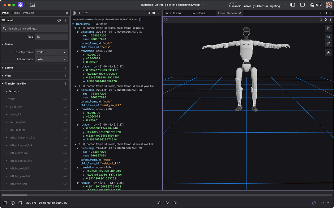
The LAFAN1 Retargeting dataset visualized using Foxglove.
The LAFAN1 Retargeting dataset visualized using Foxglove.
Code is available in the foxglove/tutorials repo.
You can also check out a short demo on youtube.