Visualizing nuScenes Data with Foxglove
Explore a rich self-driving car dataset with Foxglove's latest demo layout
We’ve shipped many visualization features to Foxglove in its first year of development.
To better showcase these features, we’ve added a sample dataset and layout for exploring the different stages of a self-driving car robotics pipeline.
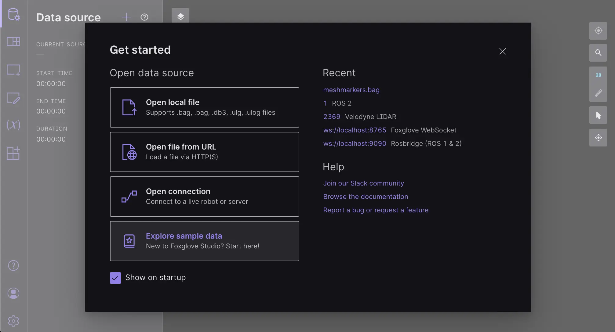
Foxglove is an open source data visualization platform for robotics and autonomy developers. Download here, and click “Explore sample data” on app load to see the sample dataset and layout.
We hope this demo will inspire you to find new ways of leveraging Foxglove for your own team’s development workflows!
A brief history of self-driving datasets
Since our own team’s history is steeped in self-driving technology, we knew we wanted our first demo to spotlight autonomous vehicles. But with the wide availability of open source self-driving datasets, we had to ask ourselves – which dataset should we choose?
The KITTI Vision benchmark, which was published in 2012 as a research paper, is considered the original publicly available dataset for autonomous vehicles. It consists of six hours of driving around a rural German town, and includes GPS coordinates, camera images, lidar returns, bounding boxes, and basic lane markers.
KITTI remained the default self-driving dataset until 2019, when Motional released nuScenes. This similarly sized dataset consisted of 1000 scenes from Boston and Singapore, and included more cameras, radar sensors, and object classification labels (32, up from KITTI’s seven). It was even accompanied by a Python library to facilitate accessing the data. This prompted Lyft to release their own dataset that same year, using a fork of the nuScenes Python library and a similar data organization. With this revived interest in public datasets, other automakers and AV companies – like Argo, Audi, Berkeley, Ford, and Waymo – followed suit.
Meanwhile, the nuScenes dataset has continued to evolve with expansion packs that added raw CAN bus data, rich semantic maps, class- and instance-level lidar segmentation annotations, planning trajectories, per-pixel image masks, and more. Taken together, this data starts to resemble the data pipelines powering today’s production autonomous vehicles, making it a great fit for demonstrating the power and flexibility of Foxglove.
nuScenes data is copyright © 2020 nuScenes and available under a non-commercial license.
A closer look at nuScenes
This section provides a technical breakdown of the nuScenes dataset. Feel free to skip to the next section if you’re not interested in these details.
To visualize the nuScenes dataset, we first have to understand the data it contains and the format it’s stored in.
Downloading the Full dataset (v1.0) contains the majority of the data: sensor captures (camera, radar, lidar), localization, and maps for the relevant regions. We then integrate the CAN bus expansion for high-frequency diagnostics, Map expansion for semantic map layers, and nuPlan maps for high-definition 2D lidar raster maps.
Once these datasets have been downloaded and unpacked into the same folder, you have all the source data used to generate our final dataset. We’ve made our own script for downloading and unpacking this data available on GitHub, so the following information is purely for reference.
Sensors
Camera images, lidar returns, and radar returns are all stored under the samples folder.
Camera images are organized into subfolders for each sensor, with individual frames stored as 1600x900 JPEG compressed images. The dataset contains “keyframes” at 2Hz (every 500ms), so that each sensor has a frame with corresponding bounding box annotations for a given timestamp. Camera images are also available outside of the keyframe captures, at roughly 12Hz.
Lidar returns are stored in the LIDAR_TOP subfolder. Individual point cloud captures are stored as .pcd.bin files, which use a simple packing of six 32-bit floating-point values (little-endian, four bytes per float) storing x, y, z, intensity, and ring values per point. The x/y/z coordinates are in the LIDAR_TOP coordinate frame.
Radar returns are also organized into subfolders for each sensor. Individual point clouds are stored in PCD v0.7 format, which uses an ASCII header followed by binary data that stores 18 different fields using different primitive types and byte widths.
Localization
Localization data lives in a single ego_pose.json file.
Each entry in the JSON array contains a timestamp in microseconds, a rotation quaternion, and a translation vector3. Although the ego pose (i.e. the car’s position) is available at a higher frequency than 2Hz, each keyframe links the sensor samples to the nearest ego pose in time.
Vehicles
The CAN bus expansion data lives as JSON files in a can_bus subfolder.
These files contain raw CAN vehicle bus data – like position, velocity, steering, lights, battery, and more – per scene. For more information, check out the CAN bus expansion README or tutorial.
Map
The nuScenes map expansion and nuPlan maps include the following:
- High-definition lidar maps
- Raster PNG files for driveable area bitmaps and lidar intensity maps
- JSON vector data for lane centerlines, lane boundaries, sidewalks, crosswalks, stop lights, and more
More information can be found in the nuScenes maps expansion tutorial.
Visualizing nuScenes with Foxglove
To visualize this data in Foxglove, we need to convert it to a format that Foxglove understands.
While Foxglove and the ROS Middleware Working Group are designing a generic recording format for robotics data (MCAP), that file specification is still a work in progress. In the meantime, the ROS bag format provides a convenient way of packaging heterogeneous data streams into a single file with type definitions, indexing, and compression.
We created a Python Jupyter Notebook to load the nuScenes data and convert each scene into a ROS bag file. Each category of data had to be converted into a ROS message type that Foxglove understands:
- Camera images – sensor_msgs/CompressedImage, sensor_msgs/CameraInfo
- Lidar and radar returns – sensor_msgs/PointCloud2
- CAN bus data – diagnostic_msgs/DiagnosticArray
- Raster maps – nav_msgs/OccupancyGrid
- Semantic maps and bounding box annotations – visualization_msgs/Marker
- Car’s position (or the ego pose) – geometry_msgs/PoseStamped, sensor_msgs/NavSatFix, tf2_msgs/TFMessage
- Additional data superimposed on camera images – foxglove_msgs/ImageMarkerArray
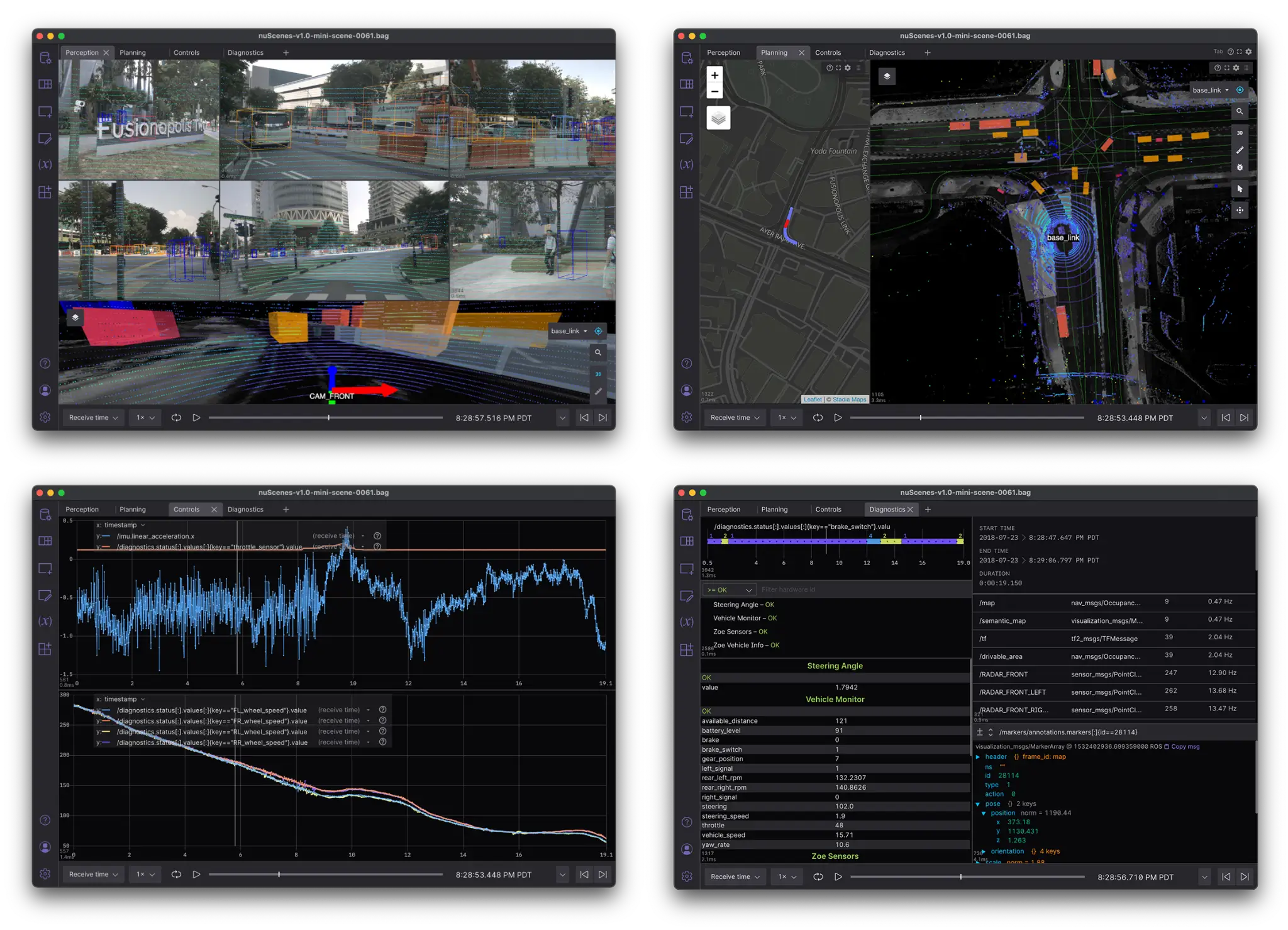
Next, we created a Foxglove layout that visualizes all this data. Since there is a lot to see in this dataset, starting with a top-level Tab panel helped organize the data around four main use cases: Perception, Planning, Controls, and Diagnostics.
Perception
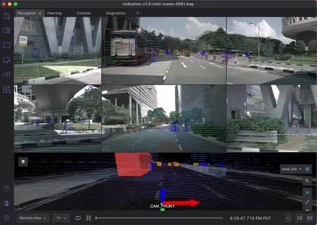
Our Perception tab focuses on sensor data, with the majority of the screen dedicated to displaying sensor_msgs/CompressedImage topics across six Image panels. The top row shows the front camera feeds; the bottom row the rear cameras. Since the Motional car has 360° camera coverage, we manually aligned the camera feeds in this layout to create two 180° views.
Each camera image also has its own pair of foxglove_msgs/ImageMarkerArray topics for the lidar points and bounding box annotations, both of which have been projected into the individual 2D camera frames.
The bottom-most panel in this tab is a 3D panel, which shows the world from the perspective of the front camera – with bounding box annotations, lidar returns, the lidar raster map, and more.
Planning
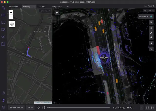
The Planning tab focuses on getting a comprehensive understanding of the whole scene, by combining a map of the area with a richly annotated 3D scene. It is split into a Map panel showing the GPS track of the vehicle, and a 3D panel in orthographic mode showing a bird’s-eye view. The 3D scene displays lane centerlines from the semantic map, our car’s pose, bounding box annotations for nearby detections, and lidar and radar point clouds.
The smooth movement of the vehicle is achieved using transform interpolation. This recently added feature allows transforms to be smoothly updated at full framerate, as long as there is a transform before and after the current time. Even though our transform messages are only published every 500ms (2Hz), we can achieve smooth movement throughout playback by publishing the transform for time t+1 at time t. Publishing future data is a luxury of post-processing an existing recording, but this can be used on live robots as well by publishing a prediction of the transform at t+1 (and overwriting it with observed data once time advances to t+1). For a deeper technical understanding of transform interpolation in robotics, the whitepaper tf: The Transform Library is a good starting point.
While the vehicle moves smoothly, everything else in the scene is moving at the publish rate of the different data streams. Lidar and radar scans come in at about 12Hz while bounding boxes are only updated at 2Hz, which appears as visibly snapping from position to position.
This tab uses the following schemas to display the various components:
sensor_msgs/NavSatFix– GPStf2_msgs/TFMessage– Coordinate frames, relative positions of the car and its sensorsvisualization_msgs/MarkerArray– Bounding box annotations, lane centersgeometry_msgs/PoseStamped– Car posesensor_msgs/PointCloud2– Radar and lidar returnsnav_msgs/OccupancyGrid– Driveable area around car, grayscale map
Controls
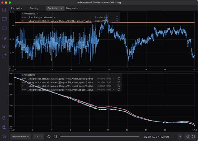
The Controls tab compares the throttle input against the vehicle’s acceleration, as measured using the Inertial Measurement Unit (IMU) and speed of all four wheels.
Each data series in the two Plot panels is specified using a message path, Foxglove’s own syntax for referencing message data.
Diagnostics
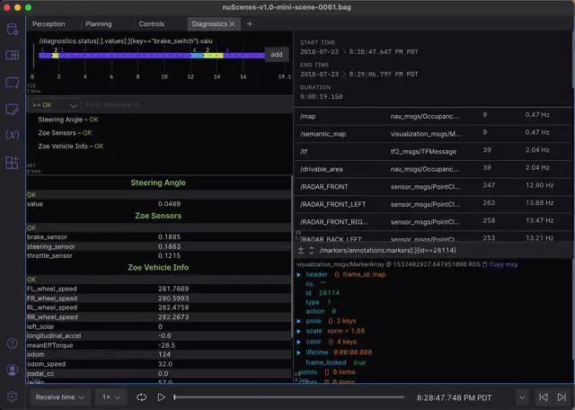
The final Diagnostics tab gives you a peek under the hood at the raw data and vehicle diagnostics.
The State Transitions panel at the top also uses message path syntax to show the brake_switch value change over time – between 1, 2, and 4. According to the nuScenes CAN documentation, possible states for this brake_switch value are 1 (pedal not pressed), 2 (pedal pressed) or 3 (pedal confirmed pressed). The unexpected 4 we see is worth investigating, if we’re interested in using this signal.
The Diagnostic Summary and Diagnostic Details panels below show the CAN bus messages formatted as a diagnostic_msgs/DiagnosticArray.
The Data Source Info panel in the top right lists all topics, schema names, and publish frequencies for our bag file.
The last view is a Raw Messages panel, used here in a rather unique way. By setting the message path to filter for a marker with a specific ID, we can monitor a single marker over time. For another creative use of this panel, try changing the message path to point to a primitive value (e.g. /markers/annotations.markers[:]{id==28114}.pose.position.x) for a single value monitor.
Further exploration
This sample dataset and layout was built to showcase the breadth of Foxglove’s newest features and to inspire you to visualize your own robotics datasets. This nuScenes example will be the first of many upcoming demos in Foxglove, all tailored to different verticals in robotics.
In the spirit of our open source philosophy, the code we used to convert the nuScenes data into ROS bag format is available on GitHub. While this was our approach, there are many ways this conversion could be extended – visualizing nuPlan trajectories, upgrading the car marker to a 3D mesh marker, or segmenting lidar points to different topics for each object classification. There is also additional nuScenes data that we could have pulled in to provide even richer visualizations.
If you have questions or ideas on how to visualize your data with Foxglove, join us in our Discord community’s #lounge channel.